class: inverse, middle, left, my-title-slide, title-slide # What are GAMs? ### Eric Pedersen ### November 2nd, 2021 --- ## Overview - A very quick refresher on GLMs - What is a GAM? - How do GAMs work? (*Roughly*) - What is smoothing? - Fitting and plotting simple models --- # A (very fast) refresher on GLMs --- ## What is a Generalized Linear model (GLM)? Models that look like: `\(y_i \sim Some\ distribution(\mu_i, \sigma_i)\)` `\(link(\mu_i) = Intercept + \beta_1\cdot x_{1i} + \beta_2\cdot x_{2i} + \ldots\)` --- ## What is a Generalized Linear model (GLM)? Models that look like: `\(y_i \sim Some\ distribution(\mu_i, \sigma_i)\)` `\(link(\mu_i) = Intercept + \beta_1\cdot x_{1i} + \beta_2\cdot x_{2i} + \ldots\)` <br /> The average value of the response, `\(\mu_i\)`, assumed to be a linear combination of the covariates, `\(x_{ji}\)`, with an offset --- ## What is a Generalized Linear model (GLM)? Models that look like: `\(y_i \sim Some\ distribution(\mu_i, \sigma_i)\)` `\(link(\mu_i) = Intercept + \beta_1\cdot x_{1i} + \beta_2\cdot x_{2i} + \ldots\)` <br /> The model is fit (not really...) by maximizing the log-likelihood: `\(\text{maximize} \sum_{i=1}^n logLik (Some\ distribution(y_i|\boldsymbol{\beta})\)` `\(\text{ with respect to } Intercept \ (\beta_0), \ \beta_1,\ \beta_2, \ ...\)` --- ## With normally distributed data (for continuous unbounded data): `\(y_i = Normal(\mu_i , \sigma_i)\)` `\(Identity(\mu_i) = \beta_0 + \beta_1\cdot x_{1i} + \beta_2\cdot x_{2i} + \ldots\)` 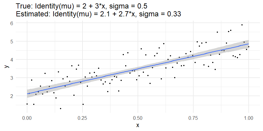<!-- --> --- ## With Poisson-distributed data (for count data): `\(y_i = Poisson(\mu_i)\)` `\(\text{ln}(\mu_i) = \beta_0 + \beta_1\cdot x_{1i} + \beta_2\cdot x_{2i} + \ldots\)` 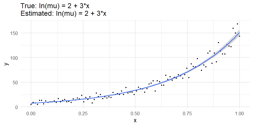<!-- --> --- # Why bother with anything more complicated? --- ## Is this linear? 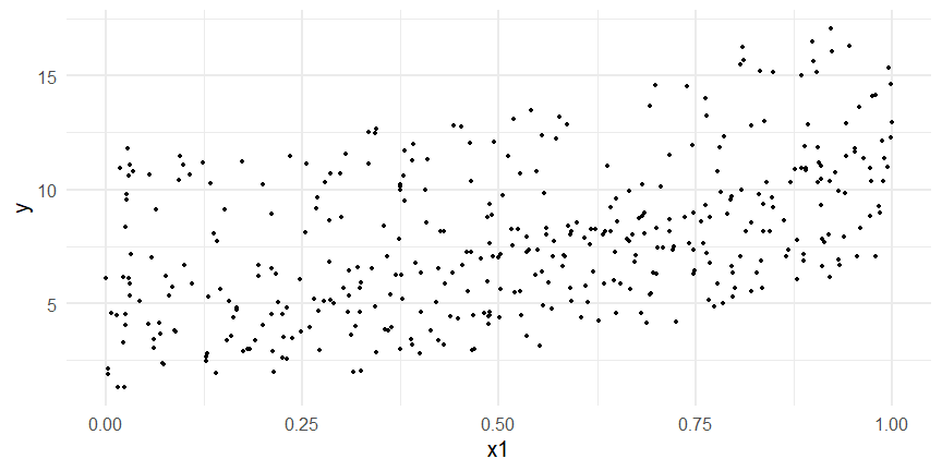<!-- --> --- ## Is this linear? Maybe? ```r lm(y ~ x1, data=dat) ``` ``` ## `geom_smooth()` using formula 'y ~ x' ``` 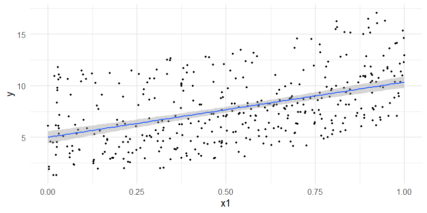<!-- --> --- # What is a GAM? The Generalized additive model assumes that `\(link(\mu_i)\)` is the sum of some *nonlinear* functions of the covariates `\(y_i \sim Some\ distribution(\mu_i, \sigma_i)\)` `\(link(\mu_i) = Intercept + f_1(x_{1i}) + f_2(x_{2i}) + \ldots\)` <br /> -- But it is much easier to fit *linear* functions than nonlinear functions, so GAMs use a trick: 1. Transform each predictor variable into several new variables, called basis functions 2. Create nonlinear functions as linear sums of those basis functions --- <img src="figures/basis_breakdown.png" width="1789" /> <!-- --> --- <!-- --> --- #This means that writing a GAM in code is as simple as: ```r mod <- gam(y~s(x,k=10),data=dat) ``` --- # You've seen basis functions before: ```r glm(y ~ I(x) + I(x^2) + I(x^3) +...) ``` -- Polynomials are one type of basis function! -- ... But not a good one. <!-- --> --- # One of the most common types of smoother are cubic splines (We won't get into the details about how these are defined) ```r glm(y ~ ns(x,df = 4)) ``` -- But even cubic splines can overfit: <!-- --> --- # How do we prevent overfitting? The second key part of fitting GAMs: penalizing overly wiggly functions We want functions that fit our data well, but do not overfit: that is, ones that are not too *wiggly*. -- Remember from before: `\(\text{maximize} \sum_{i=1}^n logLik (y_i|\mathbf{\beta})\)` `\(\text{ with respect to } Intercept, \ \beta_1,\ \beta_2, \ ...\)` --- # How do we prevent overfitting? The second key part of fitting GAMs: penalizing overly wiggly functions We want functions that fit our data well, but do not overfit: that is, ones that are not too *wiggly*. We can modify this to add a *penalty* on the size of the model parameters: `\(\text{maximize} \sum_{i=1}^n logLik (y_i|\mathbf{\beta}) - \lambda\cdot \mathbf{\beta}'\mathbf{S}\mathbf{\beta}\)` `\(= \text{maximize} \sum_{i=1}^n logLik (y_i) - \lambda\cdot \sum_{a=1}^{k}\sum_{b=1}^k \beta_a\cdot\beta_b\cdot P_{a,b}\)` `\(\text{ with respect to } Intercept, \ \beta_1,\ \beta_2, \ ...\)` --- # How do we prevent overfitting? `\(\sum_{i=1}^n logLik (y_i|\boldsymbol{\beta}) - \lambda\cdot \boldsymbol{\beta}'\mathbf{S}\boldsymbol{\beta}\)` <br /> -- The penalty `\(\lambda\)` trades off between how well the model fits the observed data ( `\(\sum_{i=1}^n logLik (y_i|\boldsymbol{\beta})\)` ), and how wiggly the fitted function is ( `\(\boldsymbol{\beta}'\mathbf{S}\boldsymbol{\beta}\)` ). <br /> -- The matrix `\(\mathbf{S}\)` measures how wiggly different function shapes are. Each type of smoother has its own penalty matrix; `mgcv` handles this. <br /> -- Some combinations of parameters correspond to a penalty value of zero; these combinations are called the *null space* of the smoother --- # How changing smoothing parameters affects the fit 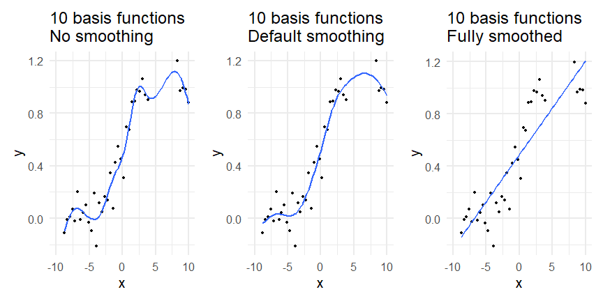<!-- --> --- # The default smoother: thin-plate regression splines We can create a penalty matrix that penalizes the squared second derivative of the curve across the range of the observed x-values: `\(\int_{x_1}^{x_n} [f^{\prime\prime}]^2 dx = \boldsymbol{\beta}^{\mathsf{T}}\mathbf{S}\boldsymbol{\beta}\)` -- <!-- --> --- 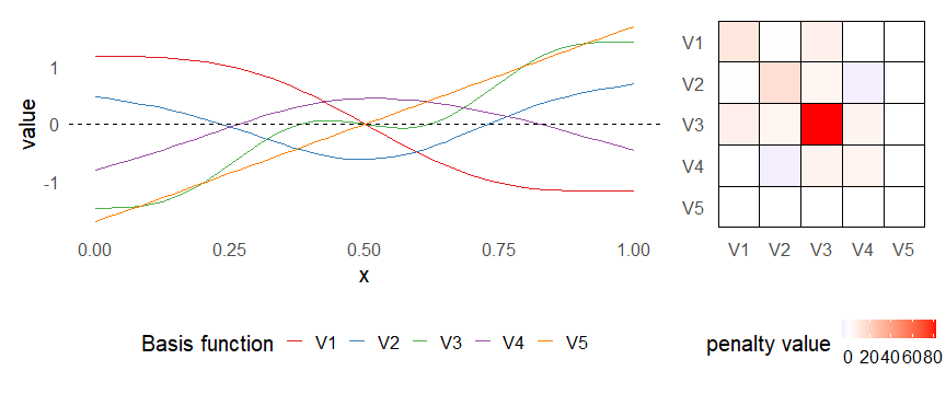<!-- --> 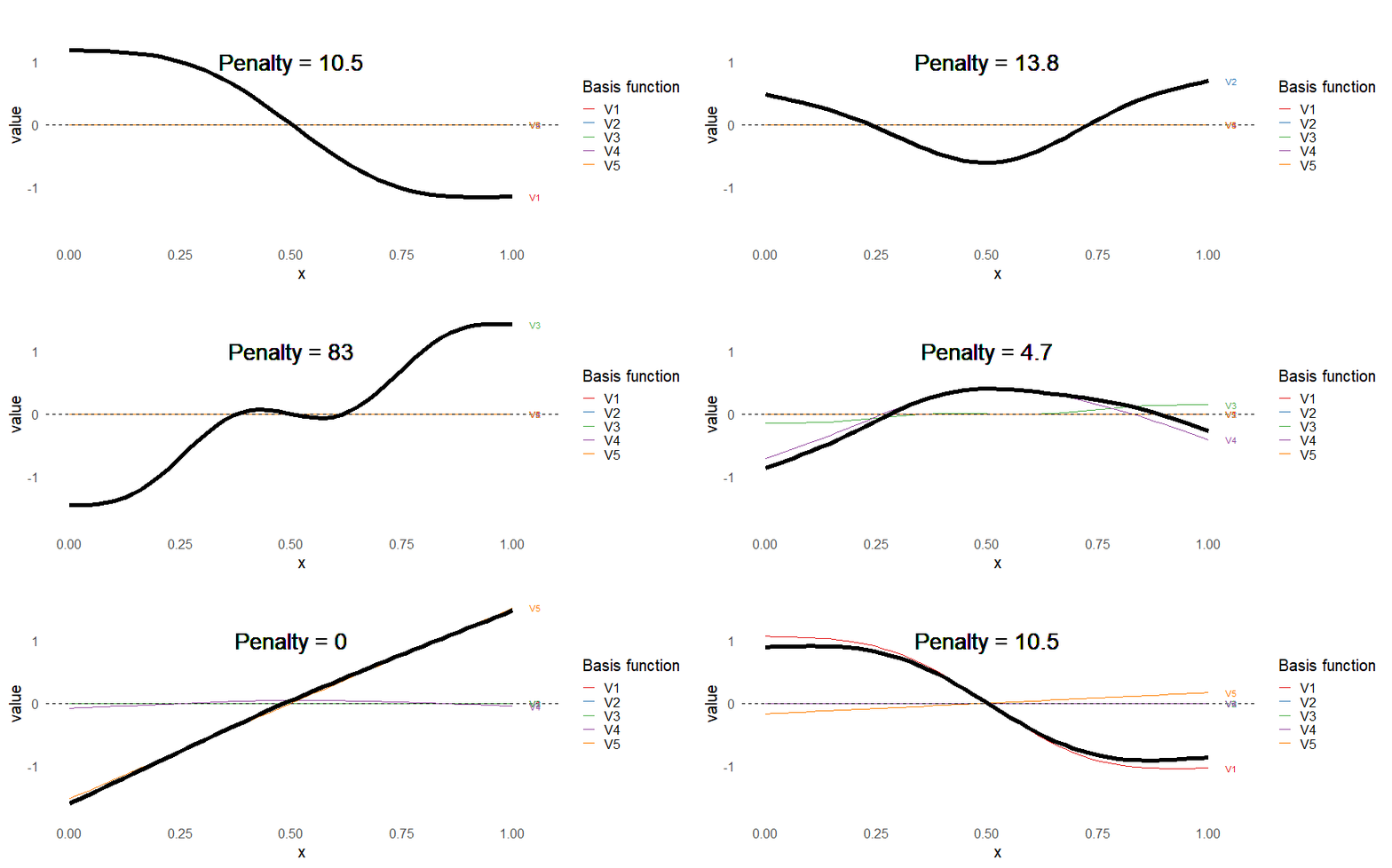<!-- --> --- # Another example basis function: cyclic smoothers Bases designed to "wrap", so the smooth will have the same value at the start and end of the function -- 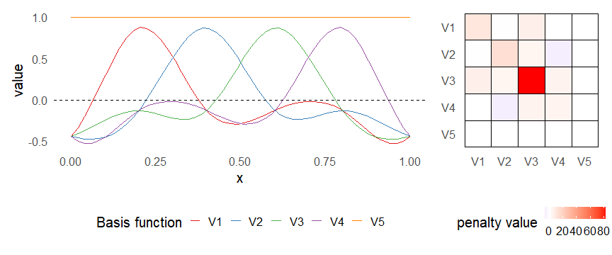<!-- --> --- 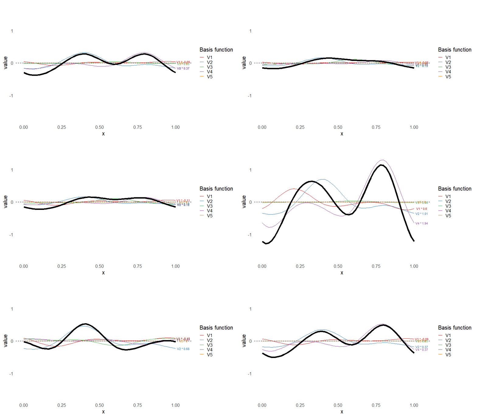<!-- --> --- # Calculating p-values, standard errors of smoothers The penalty `\(\lambda\)` also determines the *effective degrees of freedom* (EDF) of a smoother: EDF of a smooth with k basis functions ranges from a minimum of `\(k_{null}\)` (fully penalized) to `\(k\)` (fully unpenalized) 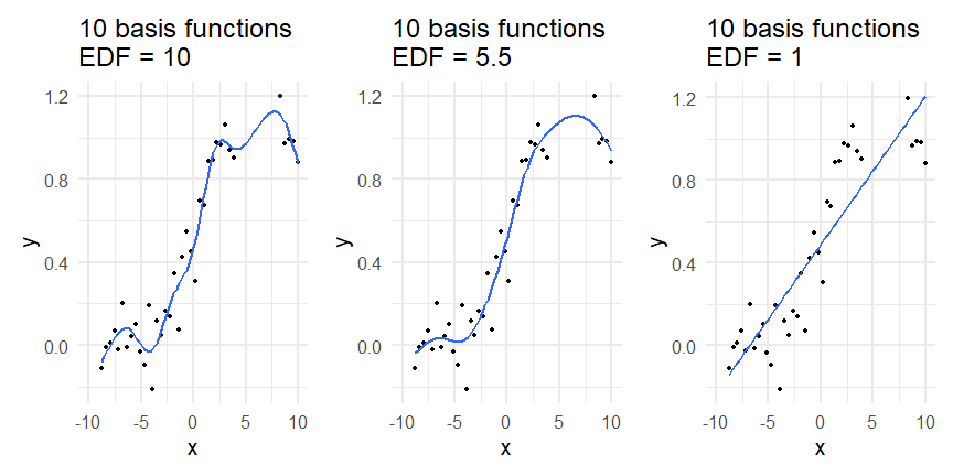<!-- --> --- # You've also (probably) already seen penalties before: Single-level random effects are another type of smoother! <img src="figures/spiderGAM.jpg" width="880" /> --- # You've also (probably) already seen penalties before: Single-level random effects are another type of smoother! You've probably seen random effects written like: `\(y_{i,j} =\alpha + \beta_j + \epsilon_i\)`, `\(\beta_j \sim Normal(0, \sigma_{\beta}^2)\)` -- * The basis functions are the different levels of the discrete variable: `\(f_j(x_i)=1\)` if `\(x_i\)` is in group `\(j\)`, `\(f_j(x_i)=0\)` if not -- * The `\(\beta_j\)` terms are the random effect estimates -- * `\(\lambda = 1/\sigma_{\beta}^2\)` and the `\(S\)` matrix for a random effect is just a diagonal matrix with `\(1\)` on the diagonal (the identity matrix), and `\(EDF = k/(1+\lambda)\)` --- # How are the `\(\lambda\)` penalties fit? * By default, `mgcv` uses Generalized Cross-Validation, but this tends to work well only with really large data sets -- * We will use restricted maximum likelihood (REML) throughout this workshop for fitting GAMs -- * This is the same REML you may have used when fitting random effects models; again, smoothers in GAMs are basically a random effect in a different hat --- # Another connection with Bayesian models .pull-left[ <img src="figures/Scooby doo - GAM - bayes.jpg" width="350px" /> ] .pull-right[ * Penalty matrices can also be viewed as *priors* on the shape of possible functions, with the penalty matrix equal to a multivariate normal prior on basis function coefficients: `\(\lambda\boldsymbol{\beta}'\mathbf{S}\boldsymbol{\beta} \rightarrow p(\boldsymbol{\beta}) = MVN(0,\lambda^{-1}\mathbf{S}^{-1})\)` ] --- # Another connection with Bayesian models .pull-left[ <img src="figures/Scooby doo - GAM - bayes.jpg" width="350px" /> ] .pull-right[ * In this context: REML estimate of `\(\lambda\)` is equivalent to the maximum a posteriori probability (MAP) estimate of the variance, with flat priors on fixed effects (i.e. unpenalized model terms) and penalties * This will be useful when we look at model uncertainties later on ] --- # To review: * GAMs are like GLMs: they use link functions and likelihoods to model different types of data -- * GAMs use linear combinations of basis functions to create nonlinear functions to predict data -- * GAMs use penalty parameters, `\(\lambda\)`, to prevent overfitting the data; this trades off between how wiggly the function is and how well it fits the data (measured by the likelihood) -- * the penalty matrix for a given smooth, `\(\textbf{S}\)`, encodes how the shape of the function translates into the total size of the penalty -- # But enough lecture; on to the live coding!