Package and workflow design
Source:vignettes/Package_and_workflow_design.Rmd
Package_and_workflow_design.RmdThe package follows an object oriented design, making use of the S4 class systems. The different classes in the package work together to produce a stepwise workflow.
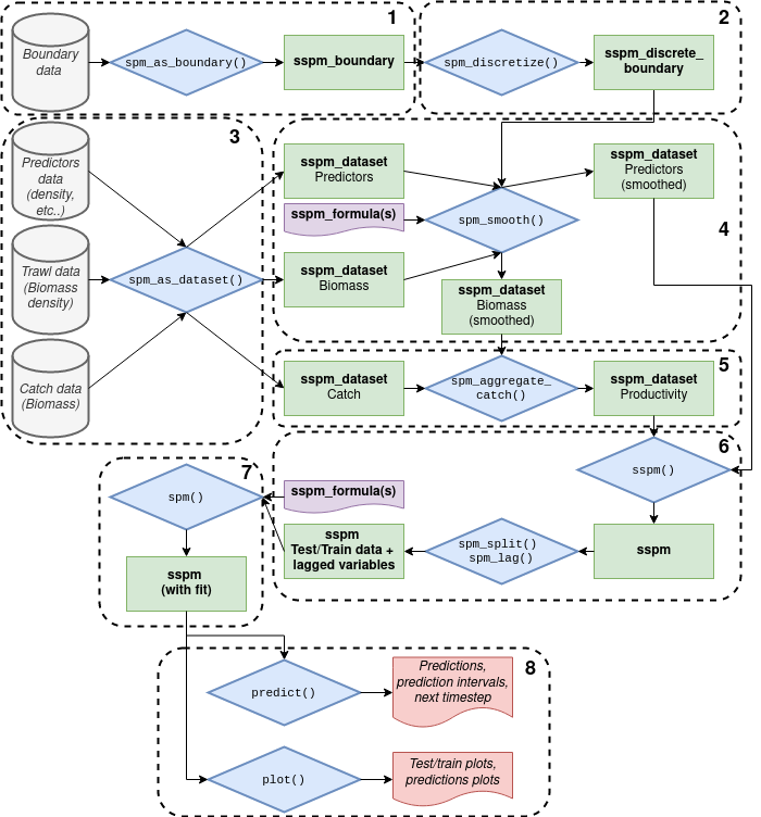
The first pillar of the package’s design is the concept of boundary data, the spatial polygons that sets the boundary of the spatial model. The boundary data is ingested into a
sspm_boundaryobject with a call tospm_as_boundary().The boundary data is then discretized into a
sspm_discrete_boundaryobject with thespm_discretize()function, dividing the boundary area into discrete patches.The second pillar is the recognition of 3 types of data: trawl, predictors, and catch (i.e. harvest). The next step in the workflow is to ingest the data into
sspm_datasetobjects via a call tospm_as_dataset().The first proper modelling step is to smooth the biomass and predictors data by combining a
sspm_dataset, and asspm_discrete_boundary. The user specifies a gam formula with custom smooth terms (see the details section of thespm_smooth()function for more details). The output is still asspm_datasetobject with asmoothed_dataslot which contains the smoothed predictions for all patches.Then, catch is integrated into the biomass data by calling
spm_aggregate_catchon the twosspm_datasetthat contains catch and smoothed biomass. Productivity and (both log and non log) is calculated at this step.The next step consists in combining all relevant datasets for the modelling of productivity (i.e. the newly created productivity dataset and the predictor(s) dataset(s)) with a call to
sspm(). Additionally, the user may apply lags to the variables withspm_lag()and determine the split between testing and training data withspm_split().The second modelling step consists in modelling productivity per se. Once again, a gam formula with custom syntax is used (see for more details).
The resulting object contains the model fit. Predictions can be obtained using the built-in
predict()method, and plots with theplot()method.